OOmmf

OOmmf is a micromagnetic simulation software. A program to simulate magnetism inside a 2D material using as a premise that the magnetization can be viewed as produced by millions and millions of spins (micro – magnetic).

This software is the product of ITL (Information Technology Laboratory) a group inside NIST (National Institute of Standards and Technology).

It started as a prototype, and they always said that it is a prototype, but in fact, it has become a popular software among the users of low performance magnetic modelling software. (In their web page you can see about 1400 papers where they use it, and that is only a part of all the papers that use it).

So, let’s go with the installation. Step one, go to the download area.

In my case, I need the windows version, 64 bits.

Source with pre-compiled 64-bit Windows executables (x64) for 64-bit Tcl/Tk 8.5.x, pkzipped archive (15 253 491 bytes).

After downloading, unzip…. and… and you cannot use it. Because this software uses TCL language and TK graphic interface. Which means (as java based programs) that you need to install
another program before running it.

For advanced people there is a long way around, which includes installing binaries and such things… Fortunately, there is a short cut for us, and is called ActiveTcl.

Is a prebuilded version of the TCL TK developing tools that will interpret the code in the OOmmf scripts.

Just go to his webpage and download the correct version for your OS. Once you have it in your computer, just run and install it.

Now you can go to your OOmmf folder an try to run oommf.tcl because of ActiveTcl, now it will run.

When you run the program, a window will appear, indicating the computer (Virgilio in my case), and the user (myself, Hector), just select them.

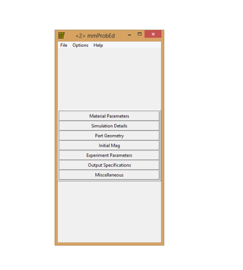
This is the main menu where all the action takes place. For now, the only interesting buttons are:

mmDisp that will open a display window to show the system under simulation.

mmProbEd that will allow you to set up the parameters of the simulation such initial state, geometry, external fields applied during the simulation, material type…

mmSolve2D this will generate the grid division of the system under simulation, that grid will be used to simulate the system as formed by thousands of micro domains

Ok, now is time for fun. But instead of using the boring examples that came with the program, we are going to go through an experimental one.

A few days ago, I used a Scanning Prove Microscopy (to remember what this is, go to this old post) to take images of a square made of Permalloy (Ni20Fe80). This is the topography image.

And this is the magnetic image.

The particularity of Py is that when disposed in thin films (this square is about 20 micrometers side and has a heigth of 20 nanometers ) induces the magnetization to lay on the main plane defined by the geometry (in this case, the magnetization is mainly laying on your screen). What we see in the magnetic image is a series of 4 lines, those lines represent domain walls between domains with magnetization pointing in different directions.

Ok ok, enough. So, how to simulate this system? To do a experimental approach, we are going to use the topography as a mask for OOmmf. A mask is a image (a *.gif file in this case) made of black and white which represents in black where the material is in the system. In our case, I took the topography image and after playing with it, I made this one (click on it and download it).

To use this image, download it and put it into OOmmf main folder (where the executable is).

Now, let’s go for the simulation. First, click on mmDisp to open a display window.

Second, click on mmProbEd, this will open the next menu.

Here we can change many things, but now we only need to change a little bit the parameters.

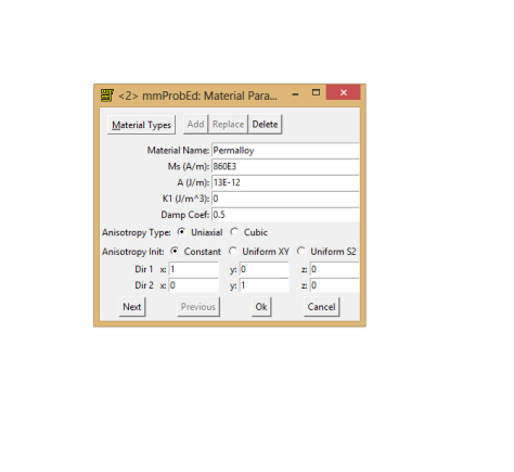
Click on Material Parameters and in material type choose Permalloy. And the only thing you need to change is setting the damping coefficient to 0.5 (This coefficient is just technical, inside Landau–Lifshitz–Gilbert equation it fixes how fast the evolution of the magnetization converges).

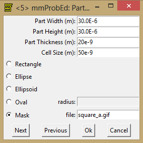
The second thing you need to change is the Part Geometry. In that menu, you need to put the size of the mask, which is about 30 micrometers, and the thickness, which is about 20 nanometers. In this case I choose 50 nanometers for the cell size. This is more a try and error process, where you have to deal with simulation time and validation of results.

And finally, the Initial Mag. Just check the initial magnetization as random.

Now go back to the main menu and click on mmSolve2D. That will create the simulation, it will appear as a tick box on the right side of the menu, click on it and you will go into the simulation menu. On that menu, the first thing you need to do is load the problem and then select what you want to show in the display window. In our case, we want the total field to be displayed every 100 iterations in the display window that we create before.

And now you are ready! Hit run or relax to see how the magnetization evolves from this random initial state.

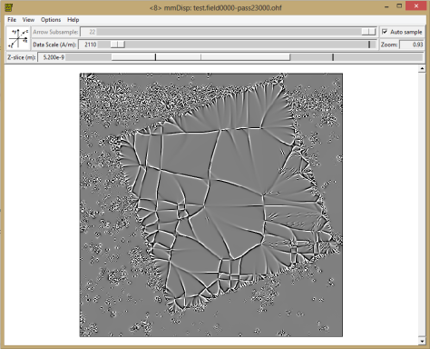
On the display window will appear something like this…

not very impressive, but if you choose the right parameters on the configuration and on the view menu…

Now the display looks more nice.

And after a long long time…. you get the stable magnetic configuration.

And that’s all for this tutorial.

.

.

.

Hey! Hold on, wait a second. That doesn’t look like the measured magnetization!

Where is the problem?

The problem is instabilities. This program tends to find solutions that are unstable in real world but are perfectly valid in simulations. How do we get rid of them?

One trick is use thermal noise (which I don’t know how to simulate in this program), the other trick is applying a gently magnetic field and reversing it. That is know as demagnetization. Sometimes it helps to get rid of unstable domains and allows the magnetization to evolve.

So, let’s go back to the mmProbEd and check Experiment Parameters. Here we can specify the applied magnetic field (direction and magnitude), and also for how many steps we want to apply it. The steps indicate how many stable solutions we want to find while the field is applied.

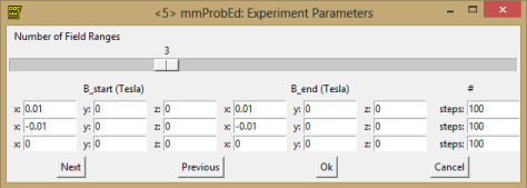
Here I have selected applying 10mT along the x-axis, first in the positive direction, later in the negative, and finally stop the field.

After setting this, repeat the simulation. The final result is now…

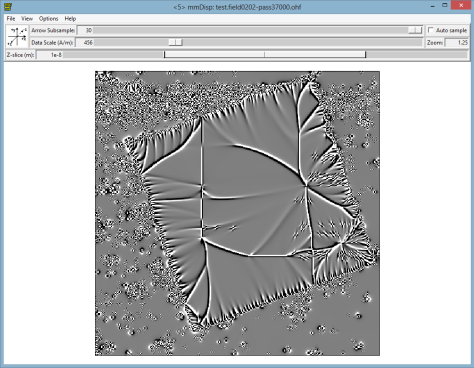
Ok, it’s still not the same, but now is closer.  A proper simulation will require even smaller cell size (wich will take several days of simulation).

.

.

.

.

What? Want more? Ok, here is a short animation I made with images of the square nanostructure taken while it was evolving in a magnetic field. Try to reproduce them with OOmmf!