KICKSTARTER PROJECT OF THE WEEK (KPW)

This week there is no project. It is the first Kickstarter of the year and I want to review the projects I considered interesting during the last year. So, first, this is the list of all the projects.

52 projects and 38 successfully funded (73% success rate)

• Linkio Funded! 60175€ pledged of 50000€ goal
• PlasmonLAB. Failed X 7027$ pledged of 21500$
• EVB. Funded! 36738$ pledged of 8000$ goal
• Seer. Funded! 160643$ pledged of 100000$ goal
• Drift Stage. Funded! 57720$ pledged of 30000$ goal
• Project Earendel Failed X 11508$ pledged of 150000$
• ScreenStick. Funded! 26949$ pledged of 6000$ goal
• Flow Funded! 12487486$ pledged of 72000$ goal
• Eight (AKA: Luna)  Funded! 1197978$ pledged of 108610$ goal
• DIY Home Automation. Funded! 5041$ pledged of 5000$ goal
• Spark Electron. Funded! 578478$ pledged of 30000$ goal
• Viper. Funded! 22579$ pledged of 20000$ goal
• Lamp. Failed X 3653$ pledged of 270000$
• Sliip Failed X 36536$ pledged of 100000$
• Ground Control. Failed X CAD4537$ pledged of CAD250000$
• Bedroom Battle. Failed X kr10705 pledged of kr40000
• GermFalcon. Funded! 4733$ pledged of 25000$ goal
• E-paper display for the Rapsberry Pi. Funded! 28593£ pledged of 10250£ goal
• SnapPower Charger. Funded! 839301$ pledged of 35000$ goal
• USB 912. Funded! 6432$ pledged of 2048$ goal
• Xbox One super battery. Failed X 1837$ pledged of 120000$
• CHIP, Funded! 2071927$ pledged of 5000$ goal
• Grut Failed X 2154€ pledged of 10000€
• For the love of Spock Funded! 662640$ pledged of 600000$ goal
• Fahrenheit 2451 – Preserve Your Data For Eternity. Funded! 45461€ pledged of 43000€ goal
• Sugru Funded! 3388150£ pledged of 1000000£ goal
• Flitchio. Failed X 6440€ pledged of 5000€
• Lunative. Funded! 43783€ pledged of 25000€ goal
• Solar Kit Box. Failed X 8683€ pledged of 25000€
• ShotBox. Funded! 106825$ pledged of 50000$ goal
• Loogun. Funded! 48718$ pledged of 40000$ goal
• Znaps. Funded! 3007370$ pledged of 120000$ goal
• KAT WALK. Funded! 149278$ pledged of 100000$ goal
• Hector Funded! 12667€ pledged of 8000€ goal
• bedjet. Funded! 1363381$ pledged of 24000$ goal
• Solar-Breeze. Funded! 408078$ pledged of 315000$ goal
• fight between EEUU and Japan. Funded! 554592$ pledged of 500000$ goal
• million mile light. Funded! 50947£ pledged of 35000£ goal
• Chief O’Brien book. Funded! 55570$ pledged of 15000$ goal
• Pugz Funded! 1433779$ pledged of 50000$ goal
• Pi-LCD Funded! 1017£ pledged of 600£ goal
• Infinite M Funded! 46327$ pledged of 35000$ goal
• Knife Edge Funded! 106998$ pledged of 10000$ goal
• Brebo. Failed X 1519€ pledged of 3000€
• Makearm. Funded! 435433$ pledged of 349750$ goal
• Felfil. Funded! 44759€ pledged of 30000€ goal
• HUI. Funded! 4407€ pledged of 2800€ goal
• Wozfans Failed X 1456$ pledged of 10000$
• STAQ Failed X 5002$ pledged of 150000$
• POD Point Funded! 321000£ pledged of 250000£ goal
• lightcan Funded! 27541€ pledged of 25000€ goal
• kGoal Failed X 72571$ pledged of 100000$

What can we learn from this projects? If we take the data from then and plot it. This is how it looks funded vs failed projects.

Interesting here is that among these projects it seems there is no intermediate projects. Either you achieved to fund the project or you fail, but there is few projects with intermediate funding. In other words, the next histogram shows that. Among these projects either they reach 100% funding or they are below 50%.

With this limited amount of data, it can be the result of randomess, or it could be something real. For now it is just interesting.

Another interesting thing is the number of backers.

There is some interesting things here. Always having into account that these results depend strongly in the small amount of projects selected. We can see that failed projects have small amount of backers, while funded projects get something in between 100 and 500 backers. Of course, there is some extreme cases where the amount of backers is huge.

But, my interpretation of this is “if you get attention into your project, you will get backers and they will make it to succeed, and in case of succeed, it will have probably between 100 and 500 backers”.

This brings us to another point. The average pledge per backer.

Here there is no big difference between the failed and the funded projects. However, it is worth noticing that the most common average pledge is below 50£ and in rare cases the average goes above 125£ per backer.

All this things brings us back to the initial graph. What is the expected revenue? (Using this non rigorous method we have been using). If the project is funded, it will have probably between 100 and 500 backers (unless it is a hit), and probably the average pledge per backer will be between 50 and 100 £. Or in other words, your project will be in the  marked area

This is a result we could have found just looking at the first graph, but we look at the other graphs to find out why there is no more failed project with funding close to the goal. And the overall conclusion is that both funded and failed projects have the same profile of backers (they put the same money in average, which means that the failed products are also valuable), however, the failed products have much less backers.

We cannot extract more conclusions, and even these ones are quite limited because of the small population used. However, they are interesting and I hope they give some hints to future projects.

Hope you find it useful.

NOTE: In order to obtain this info, I made a script to gather the data from the Kickstarter webpage. Because there is no public API, I had to code a parser that reads the info directly from the webpage. It is far from being perfect and does some mistakes. During the next months I’ll be improving it and from time to time I will present some data here. Hope you liked what you saw, even if the conclusions presented here are partially true (or completely wrong).

Music for your projects.

When you are preparing a new project (doesn’t matter if it is a game, a video, a presentation or a new home audio system), it is always good to have access to some music to use as background.

One good way of having music in your projects is by using music with creative commons license, and one good way of getting access to that music is through digccmixter.

How it works? Simply look for the type of music you need, check the type of license associated with it, download it and use it (give proper credit to authors if required).

These are the types of licenses they use in their files.

As an example, I downloaded this song:

I dunno by grapes (c) 2008 Licensed under a Creative Commons Attribution (3.0) license. http://ccmixter.org/files/grapes/16626 Ft: J Lang, Morusque

Then using media.io an MP3 online file type converter, I turned into WAV format.

Because I didn’t have any project or video at the moment, I simply created a video with my Matlab script to make spectrogram videos out of WAV files.

The final result is quite good, and notice of course that I acknowledge the music authors in the video description.

 

Moon Lander in Matlab

It has been a while since my last submission to Matlab File exchange, the popular repository of Matlab scripts done by the users.

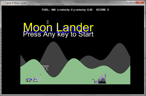
But finally it is online a new version of the Moon Lander Game.

(image credit: Héctor Corte-León)

Please, go and try it. Feel free to comment about the code. I’m here to learn and improve and to help if I can.

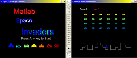
Also, remember to check my other game, Space Invaders.

(image credit: Héctor Corte-León)

St Valentine’s day

A few days ago I watched this video and though about you and how close was St Valentine’s day…

and then I start thinking… I want to make the same for you… I want to give you the most beautiful thing I can imagine… but I don’t want to harm any butterfly… and anyway, I’m not able to catch them so what I can do?

I was in a dead end, but  then I though, hey, I know quite a lot about Matlab. Maybe I can program a butterfly for her…

… and if I can make one butterfly for you, then I can make

 

2,

 

3,

.

.

.

.

or….

 

 

 

 

 

I can make a thousand!

All of them for you. Happy St Valentine’s day!

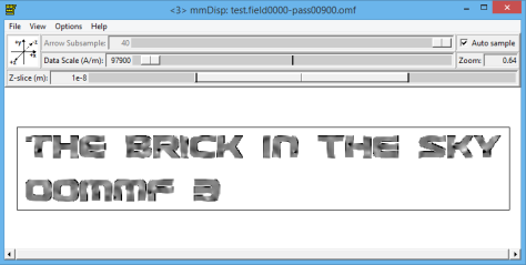
OOmmf 3

In this new OOmmf post/tutorial I want to go through the on how to define problems as files instead of using the problem editor. Again it is for 2D problems. I think this is something important if you want to optimize the usage of the program and do lots of simulations (e.g. like when trying to optimize a device geometry).

Before I start, remember to check the other 2 tutorials

OOmmf

Where I show the basics of how to set a problem and run a simulation using an image to define the geometry.

OOmmf 2

Where I describe how to save magnetization and convert the files into images to build an animation of the simulation.

So the problem for today is being able to simulate these 3 geometries which I draw using Inkscape (you can download them or draw ones yourself).

As you can see I’m changing where the wire joins the disk.

The size of the images is 4 by 2 micrometers, and the material is going to be Permalloy (magnetization along the plane of the device), 20 nm thick.

 

The names of the files are going to be:

4um_2um_0nm.png

4um_2um_250nm.png

4um_2um_500nm.png

Now for the script to run a single program. Create a txt file named example and copy this (extracted from the documentation about how to set problems as MIF files and modified for our case). We are going to simulate the first of the geometries, applying a field along the x axis from -100 mT to 100 mT.

# MIF 1.1
#
# All units are SI.
#
####################### MATERIAL PARAMETERS ############################
Ms:  800e3                 # Saturation magnetization in A/m.
A:   13e-12                # Exchange stiffness in J/m.
K1:  0.5e3                 # Anisotropy constant in J/m^3.
Anisotropy Type: uniaxial  # One of <uniaxial|cubic>.
Anisotropy Dir1: 1 0 0     # Directional cosines wrt to coordinate axes

####################### DEMAG SPECIFICATION ############################
Demag Type: ConstMag # One of <ConstMag|3dSlab|2dSlab|3dCharge|FastPipe|None>.

########################## PART GEOMETRY ###############################
Part Width:     4.0e-6    # Nominal part width in m
Part Height:    2.0e-6     # Nominal part height in m
Part Thickness: 20e-9       # Part thickness in m.
Cell Size:      20e-9     # Cell size in m.
#Part Shape:
Part Shape: mask {I:\Oommf simulations\oommf12a5rc_20120928_85_x64\oommf-1.2a5\4um_2um_0nm.png}
###################### INITIAL MAGNETIZATION ###########################
Init Mag: Random # Initial magnetization routine and parameters

###################### EXPERIMENT PARAMETERS ###########################
Field Type: Uniform
Field Range: -.100 0. 0. .100 0. 0. 20 # Start_field Stop_field Steps
Field Range: .100 0. 0. -.100 0. 0. 20
# The above applies a uniform field stepped from (-.1, 0. ,0.) to (.1,0.,0.) (Tesla), and
# back, in approximately 0.01 T steps.

Default Control Point Spec: -torque 1e-6 # Assume equilibrium has been
# reached, and step the applied field, when the reduced torque |mxh|
# drops below 1e-6.

###################### OUTPUT SPECIFICATIONS ###########################
Base Output Filename: samplerun
Magnetization Output Format: text %g # Save magnetization states

########################## MISCELLANEOUS ###############################
Randomizer Seed: 1   # Value to seed random number generator with.
User Comment: This is an example MIF file, with lots of comments.

Save the file, close the text editor and change the file format to *.mif.

As you can see the definition of the problem in this way is very similar as using mmProbEd. You can also define the problem using mmProbEd and save it as a mif.

To run this problem start Oommf open for example  mmDisp and File>Show Console

In the console simply run

Tclsh oommf.tcl batchsolve {I:\Oommf simulations\oommf12a5rc_20120928_85_x64\oommf-1.2a5\example.mif}

This will automatically run the problem and save the output in *.omf format (magnetization).

Remember OOmmf 2 post on how to convert in images the output. We run

tclsh oommf.tcl avf2ppm *.omf -config magnetic.txt -opatsub .jpg
 -filter "tclsh oommf.tcl any2ppm -format jpeg"

and with Gimp we can construct the animation.

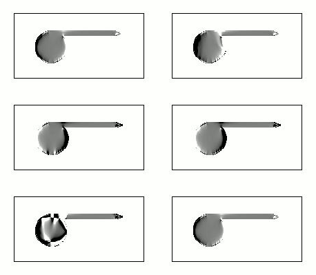
The cell size is very big (so the example will finish fast) but we can see that it worked because in the animation we can see how the colour changes in one of the ends.

Can we visualize this process and extract exactly when the transition happens? Yes we can.

At the same time as the magnetization was saved, a file named *.odt is created. This file can be opened in mmGraph in order to plot the different outputs from the problem.Remember that if you run again the same problem the vector files will be rewritten, but the odt file will not be deleted, new results will be appended.

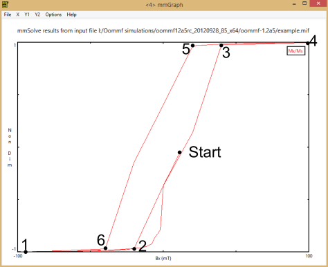
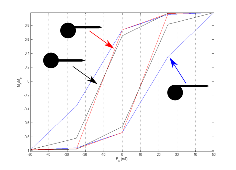
In the next graph I ploted in x the magnetic field along x and in y I ploted the magnetization along x Mx respect to the magnetization at saturation. We are interested in Mx/Ms against Bx because the jumps are going to tell us when the structure reverses magnetization.

Here is possible to see 2 effects combined, the big cell size and the few field steps. Their effect is that it is not possible to see where the transition happens.

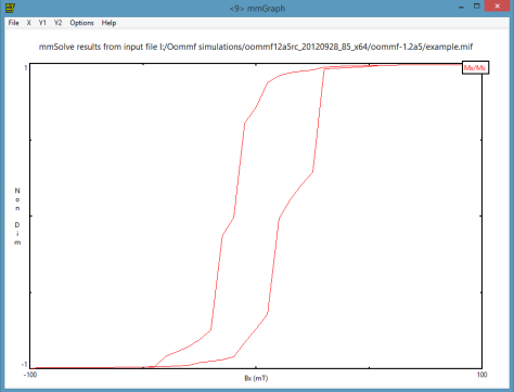
In the next graph I have double the number of field steps to show how transitions are now more clear.

Now the different transitions are more clear. Also is possible to see that is not necessary to reach 100 mT to saturate the device. Actually, 50 mT is enough. That is going to reduce quite a lot the simulations for the next part.

Before going to the last part, let me notice that is possible to open this data file in Matlab. (Remember that I have a script for uploading the vector files into Matlab)

It’s not straigth forward opening the *.odt file into Matlab, but I wrote an script that is available to download in matlabfile exchange.

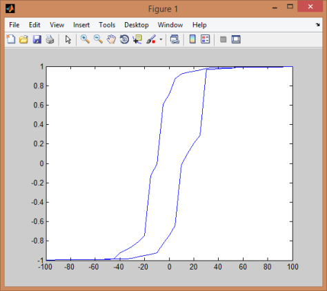
With this script you can extract the data from a *odt file and plot it in Matlab. (It will only work when the odt file corresponds to a single problem, several problems in the same odt file will produce an error).

Running the script will allow you to get the same graph and you can extract the data more easily.

Now for the last part.

My original idea was to try the batch processing available in Oommf to automatize the simulations, but it seems the batch processing has a bug with most of the Windows OS. It is something related to the usage of the ports by Oommf and the system… and it’s not easy to solve. It seems in Linux that problem doesn’t exists.

So let’s do the next part just running 3 problems one after the other.

First thing is to create 3 *.mif files as the one we just run just changing the name of the image used for the geometry and the name used for saving the files.

4um_2um_0nm.png -> 4um_2um_0nm.mif

4um_2um_250nm.png -> 4um_2um_250nm.mif

4um_2um_500nm.png -> 4um_2um_500nm.mif

Running each one of the problems as in the first example we will obtain 3 *.odt files that once opened in Matlab allow us to compare the devices. The result is shown in the next graph.Despite the simulations were made with very big cell size and few field steps, is possible to see that there is a big difference between having the joint between the nanowire and the disk in the centre or in one side.

SOAP WSDL and MATLAB

It has been a while since my last MATLAB post so…

I was trying to retrieve data from the National Weather Service  for another post when I found a protocol.

The protocol is called SOAP (Simple Object Access Protocol). In simple words, It defines an standard procedure to communicate information between different computers over internet. (I’m not an expert, so I’m basically learning while writing this).

So, let’s make it simple. Suppose we have two computers, HOME and DATA_SERVER. We have a program in HOME that wants to retrieve some data from DATA_SERVER, maybe raw data and some basic operation as counting the number of elements. How to do it? The HOME computer can send an XML document to DATA_SERVER and DATA_SERVER will read that document and execute the instructions in it. Most probably, returning some data. An XML document is simple a kind of text file that uses indentation and mixes code with normal language. Something like this:

Now, because it will be a complete mess with many different systems and programs and ways of writting code, there is an standard on how to writte that XML document, is called SOAP. SOAP describes a standard way of writting the XML document so it can be understanded by a wide range of programs, and if there is some update in the program, the XML will still work. A XML document written according to SOAP will look something like this:

Or being more specific, something like…

</pre>
<pre class="de1">POST /InStock HTTP/1.1
Host: www.example.org
Content-Type: application/soap+xml; charset=utf-8
Content-Length: 299
SOAPAction: "http://www.w3.org/2003/05/soap-envelope"

<span class="sc3"><span class="re1"><?xml</span> <span class="re0">version</span>=<span class="st0">"1.0"</span><span class="re2">?></span></span>
<span class="sc3"><span class="re1"><soap:Envelope</span> <span class="re0">xmlns:soap</span>=<span class="st0">"http://www.w3.org/2003/05/soap-envelope"</span><span class="re2">></span></span>
  <span class="sc3"><span class="re1"><soap:Header<span class="re2">></span></span></span>
  <span class="sc3"><span class="re1"></soap:Header<span class="re2">></span></span></span>
  <span class="sc3"><span class="re1"><soap:Body<span class="re2">></span></span></span>
    <span class="sc3"><span class="re1"><m:GetStockPrice</span> <span class="re0">xmlns:m</span>=<span class="st0">"http://www.example.org/stock"</span><span class="re2">></span></span>
      <span class="sc3"><span class="re1"><m:StockName<span class="re2">></span></span></span>IBM<span class="sc3"><span class="re1"></m:StockName<span class="re2">></span></span></span>
    <span class="sc3"><span class="re1"></m:GetStockPrice<span class="re2">></span></span></span>
  <span class="sc3"><span class="re1"></soap:Body<span class="re2">></span></span></span>
<span class="sc3"><span class="re1"></soap:Envelope<span class="re2">></span></span></span></pre>
<pre>

 

I’m trying to keep it as low and understandable as possible.

Now, how to create this SOAP documents?

Well, in fact there is an easy way for HOME to create the SOAP document for sending it to DATA_SERVER.

A part from SOAP, we have WSDL (Web Services Description Language). WSDL is a XML document that describes all the instruction that a machine/program can accept and how to call them. Basically WSDL is a document to tell HOME what kind of instructions to send to DATA_STORAGE inside the SOAP document. At the same time, it is standard and it’s usage can be automated, so you can have a program in HOME computer that analizes data from internet sources. If a new source appears it will have it’s own WSDL document telling you how to access it’s data using a SOAP document. You simply download that WSDL document and asks your computer to generate the code.

Ok ok, sounds nice… AN EXAMPLE PLEASE!!!!

MATLAB Real-Time currency converter

The description I just made is a little bit simple, but should be enough to understand how this things work. In the end, there is a set of nodes, paths, intermediates… that read the SOAP documents, interpret them and redirects everything.

Let’s just say that one source of WSDL documents to access several different data bases is WebserviceX.NET

In this web page you can have WSDL documents for many data bases. The one we are interested now is the currency exchange one

The currency exchange WSDL will tell our program (in this case MATLAB) how to ask for the actual currency exchange. When we click on the link… We acces a webpage with the WSDL link.

Step 1: Just copy the link to the WSDL document to use it in MATLAB: http://www.webservicex.net/CurrencyConvertor.asmx?WSDL

Now go to MATLAB. The documentation that will help us is Access Web Services Using MATLAB SOAP Functions.

Step 2: Use the WSDL file to create a MATLAB class.

createClassFromWsdl('http://www.webservicex.com/CurrencyConvertor.asmx?wsdl')

It will create a folder for the class on your working directory (it will be named @CurrencyConvertor).

Step 3: Create an object of the new class (the creation name of the class will be the name of the directory, which will have a m-file inside with the same name, the rest of m-files will be procedures to be used with the object ).

x=CurrencyConvertor

I cannot explain here what a class in MATLAB means, but suppose you want to create vectors and tell MATLAB how to work with a vector. You will define the class vector which has fields, properties etc… in the simple case, just a set of numbers. Then appart from that definitions, you define procedures to work with vectors. One procedure will be for instance how to add 2 vectors (for instance adding together the set of numbers).

Step 4: If you go into the created class directory, you will find 3 m-files, if you open them, one if to create the class, one to display the information of the WSDL and the other one called ConversionRate is to request the conversion rates. It’s just a function to be used with the object we just created “x”. And the description tells us how to use it. For instance, retrieving the conversion rate between USA Dollar and United Kingdom Pound:

ConversionRateResult = ConversionRate(x,'USD','GBP')

And the answer is 0.5948 is it correct? According to Google, it is:

Nice!

MATLAB Stock Exchange Quote  

This one will tell us how to get real data from the stock exchange.

I think many people will find this one extremely interesting.

Step 1: Get the WSDL file from WebserviceX

Step 2: As before create a class:

createClassFromWsdl('http://www.webservicex.net/stockquote.asmx?WSDL')

Step 3: Create an object of that class

value=StockQuote

and use it to get the stock value of… “IBM” (of course, you need to look for the names of the stock values, and one good place to do that is Yahoo Finances)

Step 4: Get the stock value of IBM. As before, checking the class folder we see that GetQuote.m is the file to get the data.

GetQuote(value,'IBM')

This time the answer is a string with text and values: <StockQuotes><Stock><Symbol>IBM</Symbol><Last>186.37</Last><Date>6/6/2014</Date><Time>4:01pm</Time><Change>+0.39</Change><Open>186.47</Open><High>187.65</High><Low>185.90</Low><Volume>3296900</Volume><MktCap>188.6B</MktCap><PreviousClose>185.98</PreviousClose><PercentageChange>+0.21%</PercentageChange><AnnRange>172.19 – 206.98</AnnRange><Earns>14.626</Earns><P-E>12.72</P-E><Name>International Bus</Name></Stock></StockQuotes>
This string can be scanned very easily to get only the desired data.

For the last example I’m going to use a different web. It’s called Xmethods and it’s a repository for WSDL links.

The last example is…

MATLAB to compare images in internet

Basically this is going to take 2 urls to 2 images and compare them and give a number. The closer to zero the closer are the images.

Step 1: Get the WSDL which is: http://www.quisque.com/fr/techno/eqimage/eqimage.asmx?WSDL

Step 2: Create the class and one object of the class.

createClassFromWsdl('http://www.quisque.com/fr/techno/eqimage/eqimage.asmx?WSDL')
x=CEqImage

Step 3: Compare this 3 images:

A (url: http://thegoodride.org/wp-content/uploads/2014/04/goonies_map_2010_a_l.jpg)

B (url: http://www.blogcdn.com/blog.moviefone.com/media/2010/06/gooniesmainscenes.jpg)

C (url: http://media0.giphy.com/media/ftvw5gPRJzdcc/200_s.gif)

&nAnd the code is

A_B=Compare(x,'http://thegoodride.org/wp-content/uploads/2014/04/goonies_map_2010_a_l.jpg','http://www.blogcdn.com/blog.moviefone.com/media/2010/06/gooniesmainscenes.jpg')

A_C=Compare(x,'http://thegoodride.org/wp-content/uploads/2014/04/goonies_map_2010_a_l.jpg','http://media0.giphy.com/media/ftvw5gPRJzdcc/200_s.gif')

C_B=Compare(x,'http://media0.giphy.com/media/ftvw5gPRJzdcc/200_s.gif','http://www.blogcdn.com/blog.moviefone.com/media/2010/06/gooniesmainscenes.jpg')

which gives us the results…
A_B=0.00709512367934017
A_C=0.008880839549091862
C_B=0.0068243582706561329
To be honest…. I think it is more usefull in terms of knowing if the image is exactly the same, but not so good for comparison.

Hope you like this short introduction.

.

.

.

.

.

.

What? Want more?

.

.

.

What I showed you was very nice… but It could be even better. Think about it commercially. Ignite is the answer.

Ignite is the same as WebserviceX.NET but commercial, that means that you will have access to many more data bases and information. Energy demand, currency income into companies, news headlines… but of course you have to pay to get that information. You need to use a login in your SOAP files.

OOmmf 2

One of the most visited post of all times in this blog is the OOmmf post with a quick introduction into OOmmf and the comparison between simulation and a real magnetic material images. That’s the reason for this post. I think people will like it.

Here we are going to create a simulation, store the data and create nice animations with it. And on top of that, we are going to learn how to export the simulation data into Matlab and Python.

Let’s start selecting the structure we want to simulate and the parameters.

The mask we are going to use is this one (click on it to download, and remember to put it into your ….\oommf12a5rc_20120928_85_x64\oommf-1.2a5\app\mmpe\examples folder).

And the material is going to be Permalloy.

This structure is interesting because it’s a typical structure to study Domain Wall (DW) nucleation and propagation. When we ramp the magnetic field from left to right we are going to see how a DW forms on the big pad and moves towards the needle-like end on the right.

So. Let’s go with the geometrical parameters for this structure. We are going to select them in a way that the nanowire connecting the pad with the sharp end is going to be around 150 nanometers wide. So, according to the image size, the mask is going to be 700 nanometers height and 3800 nanometers wide. The cell size is going to be 5 nanometers (for Permalloy the exchange length is 5 nanometers, so the cell must be that size or even smaller, and many published papers use 5 nanometer in the simulations).

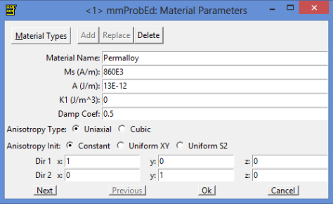
For the material we are going to select Permalloy as it comes in the program with standard parameters.

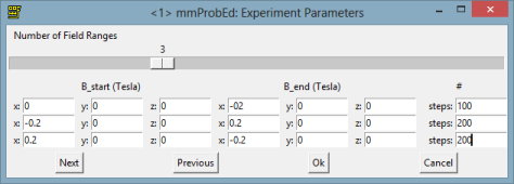
And now let’s specify the external magnetic field during the simulation. We are going to create 3 steps where the field is changing in this way:

from 0 to -200mT in x axes

from -200 to 200 in x axes

from 200 to -200 in x axes

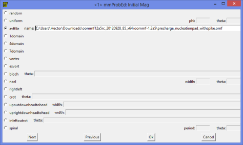
The next thing is now to select the initial magnetization. You can use a random magnetization. In our case we are going to use a previous saved file which magnetization divergence looks like this:

Just load the data file into the initial magnetization path.

Later we will explain how to save data, because this is a very useful trick to resume simulations or start from a particular state. Now the final step to prepare the problem is to select the output and change it from binary 4 to text %g. In this way the magnetization in each point will be stored as a text number. In this way is going to be quite easy to load the data into Matlab to do more analysis.

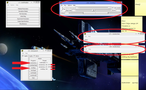
We are ready now to do the simulations, the next thing is to open a display to show the magnetization on the screen and 2 archives to save data. Remember to keep all of them on the screen, including the problem editor. Sometimes if you close the problem editor the values are reset.

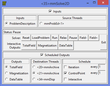
Ok, so click Solve2D, load the problem and select to visualize the magnetization on the display every 100 iterations. For the first archive select magnetization and store also every 100 iterations. For the second archive store total field every 100 iterations. Ideally we only want to save every control point, that is, when a stable magnetization is reached for every magnetic field step. But the Domain Wall propagation along the wire is a dynamic process, and we will miss it if we store on control points (I know, I did it before). And why 100? Why not every one iteration? Because I did this simulation before and it is going to take about 406934 iterations, so even saving every 100 means more than 4000 data files.

Click Run and wait…

This is going to generate screen outputs every 100 iteration steps, and save the data on every control point (each time equilibrium is reached for a set field).

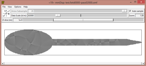
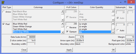
If you want to display the data while running the simulation as we do here, this is the configuration for the display. A little trick is to change the data scale on the display and reduce it. That will increase the contrast on the image.

.

.

.

.

It took me a few days finishing the simulation (not running during nigths and not at full speed (that is something I need to investigate why)), but finally you will have 1004 files generated. Half of them will look like test.field0xxx-passxxxxxx.ohf that ones are for the total field on each point of the simulation, and half of them will look like test.field0xxx-passxxxxxx.omf that ones are for the magnetization at each point.

ok. Can we actually transform these files into something we can “see” or analyse in some way? Yes, we can.

We have:

About 500 files with magnetization (*.omf).

About 500 files with total field (*.ohf).

Our options

Turn Data into Images and compose an animation.

Import data into another program and do an animation there.

Turn Data into Images and compose an animation.

Let’s try the easy route. Turn data into Images and compose an animation. To do that, on the display window File>Show Console and we start to figth with the OOmmf console. I say this because some commands will work, others not… and everything will sound weird to people like me, used to write commands in other way. Anyway. After some try and error I found that this command will turn all the .omf files in the main OOmmf folder into jpg images.

tclsh oommf.tcl avf2ppm *.omf -config magnetic.txt -opatsub .jpg
 -filter "tclsh oommf.tcl any2ppm -format jpeg"

You just type it in and it will turn all the magnetization files into jpeg images. But before doing it, remember to create a options file named (in this case) magnetic.txt It will be a text file with options for the conversion. This is how it looks like in my case.

array set plot_config {
    colormaps  { Red-Black-Blue Blue-White-Red Teal-White-Red \
            Black-Gray-White White-Green-Black Red-Green-Blue-Red }
    arrow,status       0
    arrow,colormap     Black-Gray-White
    arrow,colorcount   0
    arrow,quantity     z
    arrow,autosample   1
    arrow,subsample    10
    arrow,size         1
    arrow,antialias    1
    pixel,status       1
    pixel,colormap     Black-Gray-White
    pixel,colorcount   60
    pixel,quantity     div
    pixel,autosample   0
    pixel,subsample    1
    pixel,size         1
    misc,background    #FFFFFF
    misc,drawboundary  1
    misc,margin        10
    misc,width         1280
    misc,height        960
    misc,crop          1
    misc,zoom          0
    misc,rotation      0
    misc,datascale     13200
}

The whole explanation for these commands is in the Nist webpage here.

You can do the same with the total field data, but is quite boring. Just change omf for ohf in the comand and select arrows in the configuration file.

Once the magnetization images are created, we can remove the first 100 (remember that those correspond to the first ramping up of the field from zero to high x negative values) and the remaining 400 images can be used to create a loop in a video, because the last one and the first one will have the same magnetization and also the same external field.

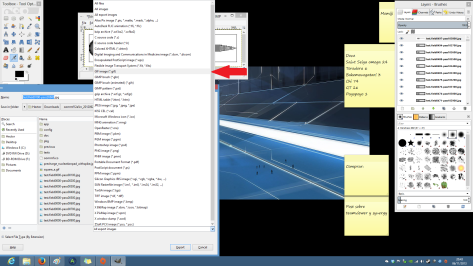
To create an animated GIF. This time we are going to use GIMP.

Just go to the webpage, download and install, it’s free and I will tell you how to use it for this.

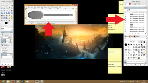
Open the program. And File>Open as layers and select all the images you have just created (first order them by date). They will appear on the layer menu and the first one will be show on the display.

And now is as simple as File>Export and select GIF on the type of file… remember to add .gif after the file name. And select export as animation.

And this is how it looks like (with low quality).

NICE!!!! It looks amazing. Notice the two kinds of Domain Walls, one when the magnetic field is saturating to the left and another one when it is saturating to the right. Also, on the pad, where there is some roughness on the surface, you can also see the Domain Wall moving like jumping, the Barkhausen effect (Domain Wall encountering defects on its way and getting pinned to them)

Now let’s try the other option.

Import data into another program and do an animation there.

To do that, I have selected Matlab and I wrote a code to import the data into it. Can be found here at the Matlab File Exchange.

Basically, what the code does is read the data files line by line, extract the data like size of the simulation, number of points used, magnetic field… And then, because we select the output to be text %g it just reads the coordinate of each vector on the vector field. To have an idea this is how a data file looks like (You can open *.omf files with Notepad and this will show).

# OOMMF: rectangular mesh v1.0
# Segment count: 1
# Begin: Segment
# Begin: Header
# Title: C:/Users/Hector/Downloads/oommf12a5rc_20120928_85_x64/oommf-1.2a5/test.field0000-pass03369.omf
# Desc: Field Index: 0 
# Desc: Applied field (T): 0 0 0 
# Desc: Iteration: 3369 
# Desc: Time (s): 1.8747579070869034e-9 
# Desc: |m x h|: 0.092583929421348854 
# Desc: User Comment: 
# meshtype: rectangular
# meshunit: m
# xbase: 2.5e-009
# ybase: 2.5e-009
# zbase: 1e-008
# xstepsize: 5e-009
# ystepsize: 5e-009
# zstepsize: 2e-008
# xnodes: 400
# ynodes: 100
# znodes: 1
# xmin: 0
# ymin: 0
# zmin: 0
# xmax: 2e-006
# ymax: 5e-007
# zmax: 2e-008
# valueunit: A/m
# valuemultiplier: 800000
# ValueRangeMinMag: 1e-8
# ValueRangeMaxMag: 1.0
# End: Header
# Begin: Data Text
-0 0 0
0 0 -0
-0 0 -0
-0.263872 -0.417373 0.000337065
-0.238721 -0.433818 0.000330522
-0.211667 -0.449099 0.000320794
-0.182926 -0.462911 0.000308174
-0.152747 -0.474998 0.000293057
-0.121395 -0.485153 0.000275874
# End: Data Text
# End: Segment

I cut down part of the data to make it fit. Notice the vectors because they have 3 coordinates, but notice they are not in the place they occupy in the simulation. To arrange them in the correct order you need to extract the data of number of x y and z nodes.

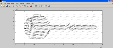
If you want to download and try my code, do it. Once you have the data on Matlab the limit is your imagination. This is how some of it will look alike.

And this is all for now. Hope you like it. Next time more.

Star Destroyer over London

Fra

Queen + Matlab + Me

I made another animated spectrum and finally post the code to Matlab FileExchange.

I want to stay on world top 500. So download it! :)