Screentendo

Screentendo lets you turn any image on your screen into a Super Mario Bros level.

Unfortunately it is only for MAC.

Embed MS-DOS games.

We have mention many times the Internet Archive, and how it keeps a database of movies, music, games… specially, MS-DOS games. Well, now it seems it is possible to embed the MS-DOS games into tweets, and yes, into webpages too. So, I use this opportunity to put in one place some of the MS-DOS games I love.

Like Prince of Persia?

I was very bad with the Prince of Persia and never managed to finish it. But I was quite good with the Great Escape, and manage to escape several times (at that point I didn’t knew English at all).

I have to admit that I never played this game to the end until a couple of weeks ago. Gateway is not only a game, but the first novel of the Heechee saga (which I love), written by Frederik Pohl. The game is nice, but quite linear, and at some points it is easy to understand what to do, but in other parts there is no other way around, you need to check a walkthrough.

This one has survived the years and nowadays is still playable in most smartphones…. although, with different names. Enjoy Bust-A-move.

Obviously, any list can’t be complete without Pac-Man.

There are more games, but it will be too much for a single post, so I will finish this small list with a classic. SimCity.

Leaked Star Wars Episode VII Filmset Footage!

Ok ok, it is not, but it is extremely funny.

Mythbusters: Star Wars Special

Michael Paul Smith and Forced Perspective.

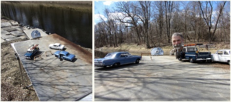
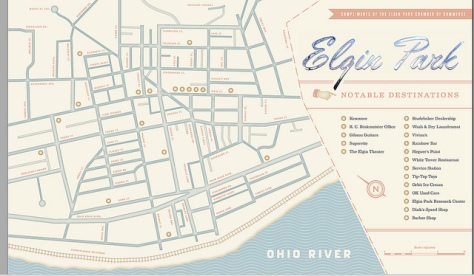
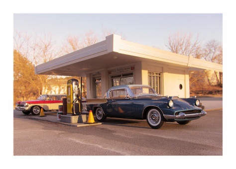
Enjoy Paul Smith and his dioramas made with model cars and forced perspective.

He has been using this technique to recreate a fantasy town called Elgin Park.

And for about 25 years he has imaged all kind of situations.

You can access his interview at fstoppers here.

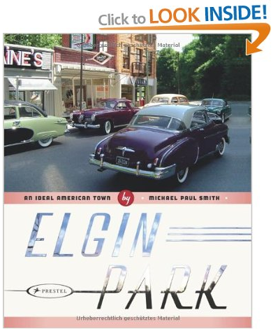
And if you like it, there is a book with all the events happening at Elgin Park.

OOmmf 2

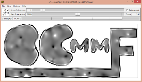
One of the most visited post of all times in this blog is the OOmmf post with a quick introduction into OOmmf and the comparison between simulation and a real magnetic material images. That’s the reason for this post. I think people will like it.

Here we are going to create a simulation, store the data and create nice animations with it. And on top of that, we are going to learn how to export the simulation data into Matlab and Python.

Let’s start selecting the structure we want to simulate and the parameters.

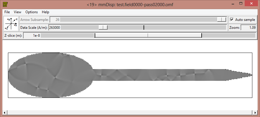
The mask we are going to use is this one (click on it to download, and remember to put it into your ….\oommf12a5rc_20120928_85_x64\oommf-1.2a5\app\mmpe\examples folder).

And the material is going to be Permalloy.

This structure is interesting because it’s a typical structure to study Domain Wall (DW) nucleation and propagation. When we ramp the magnetic field from left to right we are going to see how a DW forms on the big pad and moves towards the needle-like end on the right.

So. Let’s go with the geometrical parameters for this structure. We are going to select them in a way that the nanowire connecting the pad with the sharp end is going to be around 150 nanometers wide. So, according to the image size, the mask is going to be 700 nanometers height and 3800 nanometers wide. The cell size is going to be 5 nanometers (for Permalloy the exchange length is 5 nanometers, so the cell must be that size or even smaller, and many published papers use 5 nanometer in the simulations).

For the material we are going to select Permalloy as it comes in the program with standard parameters.

And now let’s specify the external magnetic field during the simulation. We are going to create 3 steps where the field is changing in this way:

from 0 to -200mT in x axes

from -200 to 200 in x axes

from 200 to -200 in x axes

The next thing is now to select the initial magnetization. You can use a random magnetization. In our case we are going to use a previous saved file which magnetization divergence looks like this:

Just load the data file into the initial magnetization path.

Later we will explain how to save data, because this is a very useful trick to resume simulations or start from a particular state. Now the final step to prepare the problem is to select the output and change it from binary 4 to text %g. In this way the magnetization in each point will be stored as a text number. In this way is going to be quite easy to load the data into Matlab to do more analysis.

We are ready now to do the simulations, the next thing is to open a display to show the magnetization on the screen and 2 archives to save data. Remember to keep all of them on the screen, including the problem editor. Sometimes if you close the problem editor the values are reset.

Ok, so click Solve2D, load the problem and select to visualize the magnetization on the display every 100 iterations. For the first archive select magnetization and store also every 100 iterations. For the second archive store total field every 100 iterations. Ideally we only want to save every control point, that is, when a stable magnetization is reached for every magnetic field step. But the Domain Wall propagation along the wire is a dynamic process, and we will miss it if we store on control points (I know, I did it before). And why 100? Why not every one iteration? Because I did this simulation before and it is going to take about 406934 iterations, so even saving every 100 means more than 4000 data files.

Click Run and wait…

This is going to generate screen outputs every 100 iteration steps, and save the data on every control point (each time equilibrium is reached for a set field).

If you want to display the data while running the simulation as we do here, this is the configuration for the display. A little trick is to change the data scale on the display and reduce it. That will increase the contrast on the image.

.

.

.

.

It took me a few days finishing the simulation (not running during nigths and not at full speed (that is something I need to investigate why)), but finally you will have 1004 files generated. Half of them will look like test.field0xxx-passxxxxxx.ohf that ones are for the total field on each point of the simulation, and half of them will look like test.field0xxx-passxxxxxx.omf that ones are for the magnetization at each point.

ok. Can we actually transform these files into something we can “see” or analyse in some way? Yes, we can.

We have:

About 500 files with magnetization (*.omf).

About 500 files with total field (*.ohf).

Our options

Turn Data into Images and compose an animation.

Import data into another program and do an animation there.

Turn Data into Images and compose an animation.

Let’s try the easy route. Turn data into Images and compose an animation. To do that, on the display window File>Show Console and we start to figth with the OOmmf console. I say this because some commands will work, others not… and everything will sound weird to people like me, used to write commands in other way. Anyway. After some try and error I found that this command will turn all the .omf files in the main OOmmf folder into jpg images.

tclsh oommf.tcl avf2ppm *.omf -config magnetic.txt -opatsub .jpg
 -filter "tclsh oommf.tcl any2ppm -format jpeg"

You just type it in and it will turn all the magnetization files into jpeg images. But before doing it, remember to create a options file named (in this case) magnetic.txt It will be a text file with options for the conversion. This is how it looks like in my case.

array set plot_config {
    colormaps  { Red-Black-Blue Blue-White-Red Teal-White-Red \
            Black-Gray-White White-Green-Black Red-Green-Blue-Red }
    arrow,status       0
    arrow,colormap     Black-Gray-White
    arrow,colorcount   0
    arrow,quantity     z
    arrow,autosample   1
    arrow,subsample    10
    arrow,size         1
    arrow,antialias    1
    pixel,status       1
    pixel,colormap     Black-Gray-White
    pixel,colorcount   60
    pixel,quantity     div
    pixel,autosample   0
    pixel,subsample    1
    pixel,size         1
    misc,background    #FFFFFF
    misc,drawboundary  1
    misc,margin        10
    misc,width         1280
    misc,height        960
    misc,crop          1
    misc,zoom          0
    misc,rotation      0
    misc,datascale     13200
}

The whole explanation for these commands is in the Nist webpage here.

You can do the same with the total field data, but is quite boring. Just change omf for ohf in the comand and select arrows in the configuration file.

Once the magnetization images are created, we can remove the first 100 (remember that those correspond to the first ramping up of the field from zero to high x negative values) and the remaining 400 images can be used to create a loop in a video, because the last one and the first one will have the same magnetization and also the same external field.

To create an animated GIF. This time we are going to use GIMP.

Just go to the webpage, download and install, it’s free and I will tell you how to use it for this.

Open the program. And File>Open as layers and select all the images you have just created (first order them by date). They will appear on the layer menu and the first one will be show on the display.

And now is as simple as File>Export and select GIF on the type of file… remember to add .gif after the file name. And select export as animation.

And this is how it looks like (with low quality).

NICE!!!! It looks amazing. Notice the two kinds of Domain Walls, one when the magnetic field is saturating to the left and another one when it is saturating to the right. Also, on the pad, where there is some roughness on the surface, you can also see the Domain Wall moving like jumping, the Barkhausen effect (Domain Wall encountering defects on its way and getting pinned to them)

Now let’s try the other option.

Import data into another program and do an animation there.

To do that, I have selected Matlab and I wrote a code to import the data into it. Can be found here at the Matlab File Exchange.

Basically, what the code does is read the data files line by line, extract the data like size of the simulation, number of points used, magnetic field… And then, because we select the output to be text %g it just reads the coordinate of each vector on the vector field. To have an idea this is how a data file looks like (You can open *.omf files with Notepad and this will show).

# OOMMF: rectangular mesh v1.0
# Segment count: 1
# Begin: Segment
# Begin: Header
# Title: C:/Users/Hector/Downloads/oommf12a5rc_20120928_85_x64/oommf-1.2a5/test.field0000-pass03369.omf
# Desc: Field Index: 0 
# Desc: Applied field (T): 0 0 0 
# Desc: Iteration: 3369 
# Desc: Time (s): 1.8747579070869034e-9 
# Desc: |m x h|: 0.092583929421348854 
# Desc: User Comment: 
# meshtype: rectangular
# meshunit: m
# xbase: 2.5e-009
# ybase: 2.5e-009
# zbase: 1e-008
# xstepsize: 5e-009
# ystepsize: 5e-009
# zstepsize: 2e-008
# xnodes: 400
# ynodes: 100
# znodes: 1
# xmin: 0
# ymin: 0
# zmin: 0
# xmax: 2e-006
# ymax: 5e-007
# zmax: 2e-008
# valueunit: A/m
# valuemultiplier: 800000
# ValueRangeMinMag: 1e-8
# ValueRangeMaxMag: 1.0
# End: Header
# Begin: Data Text
-0 0 0
0 0 -0
-0 0 -0
-0.263872 -0.417373 0.000337065
-0.238721 -0.433818 0.000330522
-0.211667 -0.449099 0.000320794
-0.182926 -0.462911 0.000308174
-0.152747 -0.474998 0.000293057
-0.121395 -0.485153 0.000275874
# End: Data Text
# End: Segment

I cut down part of the data to make it fit. Notice the vectors because they have 3 coordinates, but notice they are not in the place they occupy in the simulation. To arrange them in the correct order you need to extract the data of number of x y and z nodes.

If you want to download and try my code, do it. Once you have the data on Matlab the limit is your imagination. This is how some of it will look alike.

And this is all for now. Hope you like it. Next time more.

Lego Adeventure Time BMO Raspberry Pi

And here are the videos.

Super Mario Bros.

Patito!!

I found this pet I made long time ago…

Chiptunes

This is a short exploration into chiptunes.

Let’s start with this, you will enjoy it. Portal 2 ending theme covered with 8 bit music.

Yes, that’s it, this post is about 8-bit music. Becuase I found a great editor, it’s called Farmitracker.

And what does this program? FamiTracker is a free Windows tracker for producing music for the NES/Famicom-systems. And the most interesting part is it’s NSF-file exporting. That allows music created in this tracker to be played on the real hardware, or even for for use in your own NES-applications. O_O Nice nice!!

To get this program, just go to the downloads webpage and get the source of the latest version. Unzip and install.

And since I’m terrible with music, here you have some tutorials. Enjoy them!

There is a nasty noise during all the video (crappy PC mirophone).

This guy know what he is doing.

The funny thing is that this sounds better than many actual games!!

And the last video.

And now, I gave you a short list of 8-bit composers to inspire yourselves.

Nullsleep. Electronic musician whit many actuations over the world. Not only dedicated to 8-bit covers for games, but have some songs.

RushJet1 His pictures says everything. Has many covers and you can download them in it’s webpage.

Tsu Ryu. Descibed as Electronic/Chiptune musician and cartoonist. doesn’t have music on his webpage, but have a very active youtube channel with nice music, like this.

Jake Kaufman. This is a big man in this busines. He has his own Wikipedia page. His webpage is a very interesting blog with many entries. Take one minute or two to check it out.

C-jeff. It’s not the kind of music you will find in games, but it’s nice. he is also one of the founders of

And I’m not sure about what it is, but have things as cool as this two (listen to the tracks).

And this one:

And this one is part of a project called Noise Channel, a radio channel to explore chiptune music.

And that’s all for today. Want more? Here is more!!